CS 221 Fall 2011 Problem Set 5

CS 221 Fall 2011 Solutions to Problem Set 5

Problem 1: Solving Nonlinear Equations

(Here is an Excel spreadsheet with solutions to all three parts.)

Part a.

Using Excel it is a simple matter to set up the equation and then use Goal Seek to find the solution. With MATLAB, we first create a function distance, which corresponds to the equation:

function d = distance(v, theta)
   th = theta * pi/180; % Convert to radians
   d = (v^2 / 9.8) * sin(2*th);
end

Then we define a function target900(theta), that simply calls distance() with the givens of the problem (namely, 100 m/s initial velocity and 900 m distance), which evaluates to 0 at the solution:

function x = target900(theta)
  x = distance(100, theta) - 900;
end

(We could also implement everything in one function, but separating them is less error-prone and therefore better programming practice.)

Then we just call fzero() with this latter function and a guess:

>> fzero(@target900, 25)
 ans =
    30.9423

This is one answer; since the maximum distance occurs at 45 degrees, there might be another; we try a different initial guess:

>> fzero(@target900, 75)
 ans =
    59.0577 
>>

There are thus two solutions, about 31° and about 59°. (Excel gives the same solutions.)

Part b.

This time we'll just define one special-purpose function, which returns zero when x is the fifth root of 200:

function Delta = prob1b(x)
  Delta = x.^5 - 200;
end

And then use fzero():

>> fzero(@prob1b,3)
ans =
    2.8854
>>

So the fifth root of 200 is 2.8854.

Part c.

This time we'll again use two functions so we can keep things straight; we encode the Van der Waals equation directly:

function P = van_der_Waals(n,V,TC)
  T = TC + 273.15; % Convert temp to Kelvin
  R = 0.08206;     % Gas constant (given)
  a = 1.39;        % Materials constants for N
  b = 0.03919; 
  P = (n*R*T) / (V-b) - (n^2 * a) / V^2;
end

And a second one that goes to zero as pressure goes to 13.5:

function y = prob1c(V)
  y = van_der_Waals(1.5, V, 25) - 13.5;
end

Calling fzero() yields:

>> fzero(@prob1c,12)
ans =
    2.6722

Excel gives the same result.

Problem 2: Solving Systems of Linear Equations

Part a.

After creating the arrays A and b, we left-divide b by A:

>> x = A\b
>>   19.9939
     29.9204
      0.9773
      0.0139
     -2.9994
>>

Part b.

>> load A.txt
>> load b.txt
>> x = A\b
x =
    1.0000
    2.0000
    3.0000
    4.0000
    5.0000
    6.0000
    7.0000
    8.0000
    9.0000
   10.0000
>>

Problem 3: Curve-fitting

Part a.

First we want to rearrange the equation into the linear form R = mT + b. When we do, we get (substituting 20 for T₀):
R = R₀αT + R₀(1-20α)

Now, if we fit a line to the given R-vs.-T data (using polyfit()), we will get the two coefficients, m and and b. We can then calculate: m = R₀ α
b = R₀(1 – 20α)

Rearranging, we get: R₀ = m/α
α = m/(b+20m))

So:

>> T = [20 100 180 260 340 420 500];      % Observed temperatures
>> R = [500 676 870 1060 1205 1410 1565]; % Observed resistance
>> c = polyfit(T, R, 1)             % Caculate best linear fit 
c =
    2.2312  460.7321
>> plot(T,R, '*', T, polyval(c,T))

Now, with m=c(1) and b=c(2), we can compute R₀ and α:

>> alpha = c(1)/(c(2) + 20*c(1));
>> R0 = c(1)/alpha;
>> plot(T,R,'*',T,R0*(1+alpha*(T-20)));
>>

And the plot confirms an excellent fit with the data. Just to be sure, we do a goodness-of-fit test, by fitting a line to the measured and predicted R values:

>> RR = R0*(1+alpha*(T-20));
>> polyfit(R,RR,1)
ans =
    0.9989    1.1629
>>

This is a very good fit.

Part b.

We first save the given file and rename it dat.txt, and put it in two appropriately-named vectors:

load dat.txt;
u = dat(:,1);
V = dat(:,2);

Now, if u = Ae^BV, we can take the log of both sides and get ln(u) = ln(A) + BV — according to the pattern in the second row of the table in the assignment. This is of the form y = mx + b, but with ln(u) instead of y, B instead of m, and ln(A) instead of b. We need to transform the data so we can solve for m and b with polyfit(); we have to give it ln(u) instead of u:

F = polyfit(V, log(u), 1)
F =
    6.5133  -45.1425
>>

Now we know the value of m and b. Now B = m, but to get A we have to exponentiate b:

>> B = F(1);
>> A = exp(F(2));

Now we can plot the function and data:

>> plot(V,u,'*',V,A*exp(B*u));

The plot looks funny because the values of the independent variable are not sorted in increasing order. We can sort the original matrix (use sortrows(dat,2) to sort on the second column) and plot again, or just do a goodness-of-fit test:

>> polyfit(u,A*exp(B*V),1)
ans =
    1.0388   -1.2599

This confirms a pretty good fit. (Note that the regression methods do not depend on the data being sorted in any way; the data is simply considered as a set of pairs. For plotting, however, it is useful to have the data sorted on the independent variable.)

Part c.

First, we plot the data to get an idea of the shape:

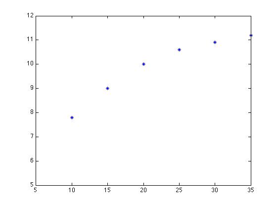
>> Age = [5:5:35];  % from 5 to 35 by 5's
>> Height = [5.2 7.8 9 10 10.6 10.9 11.2];
>> plot(Age, Height, '*') % Graph shows that the relation is nonlinear

This gives:

It is clearly nonlinear. It is also not a pure exponential. We can try a power-law form: y = bx^m, which becomes ln(y) = m ln(x) + ln(b) when we take the log of both sides. So to use polyfit, we have to give it the logs of both Age and Height:

>> F = polyfit(log(Age), log(Height), 1)
F = 
    0.3888    1.0961     
>> m1 = F(1)
m1 =
    0.3888
>> b1 = exp(F(2))
b1 = 
    2.9924

We plot it, using a more finer-grained x-axis to get a better fit:

>> Age_range = [min(Age)/2:0.05:max(Age)*1.25];
>> H1 = b1 * Age_range .^ m1;
>> plot(Age, Height, '*', Age_range, H1)

This gives:

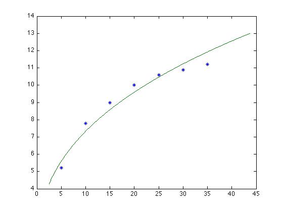
Which is OK, but looks like it may not flatten out fast enough. The goodness-of-fit test is not bad.

>> polyfit(Height,b1*Age.^m1,1)
ans =
    1.0239   -0.2199

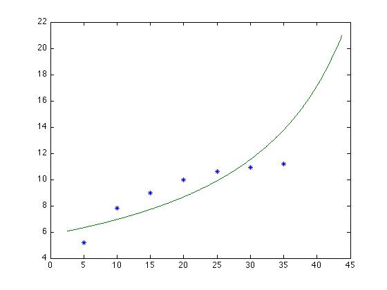
Exponential curves never have this shape, so we need not bother with that form. Although it seems unlikely that the third form will fit either, we give it a try: y = 1/(mx + b) or 1/y = mx + b. Again, we transform the data by taking the reciprocal before giving it to polyfit():

>> F = polyfit(Age, 1./Height, 1)
F =
   -0.0028    0.1723
>> m2 = F(1);
>> b2 = F(2);
>> H2 = 1./(m2 * Age_range + b2);
>> plot(Age, Height, '*', Age_range, H2)

This gives:

Which does not look like a good fit.

Finally, we try the form y = (mx)/(x+b), which transforms into 1/y = b/mx + 1/m. For this we have to give the reciprocal of both Age and Height to polyfit(); we get back as coefficients (i.e., F(1) and F(2)) b/m and 1/m, respectively. This means that m = 1/F(2) and b = m*F(1).

>> F = polyfit(1./Age,1./Height,1)
F =
    0.6025    0.0706
>> m3 = 1/F(2)
m3 =
   14.1546
>> b3 = m3*F(1)
b3 =
    8.5285
>> H3 = (m3 * Age_range) ./ (Age_range + b3);
>> plot(Age,Height,'*',Age_range,H3)

The plot looks like this: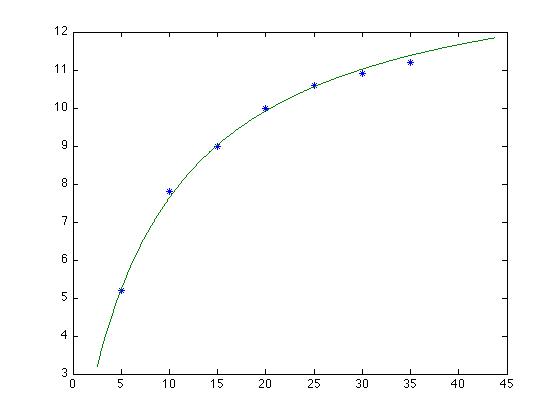

This looks like an excellent fit. To be sure, we check the goodness-of-fit:

>> polyfit(Height,(m3*Age)./(Age + b3),1)
ans =
    1.0195   -0.1692
>>

This is the best fit yet, and so we conclude that tree height varies with age according to:
height = (14.1546 * age)/(age + 8.5285)