CS 221 Fall 2011 Problem Set 3

CS 221 Fall 2011 Solutions to Problem Set 4

Problem 1: fixpoint() function

See fixpoint.m. You should have turned in something like it, except that this one includes two different checks for divergence—one based on slope and one based on whether guesses are getting further apart. Here is a version that takes a fourth parameter, which controls whether it prints anything out (for debugging purposes).

Problem 2: Using root-finding methods

The problem involved finding roots of two different equations (three, counting different parameter values), using three different methods.

Sphere volume problem with R=4, V=30.

(a) MATLAB Methods. The first thing to do is get the function into a form so that when f(x)=0, x is a solution to the problem. Since we want a height (h) that gives a particular volume (V), and since the equation relates h, V, and R, we need to write a function based on the given equation that will return 0 for the value of h that would yield V=30 (with R=4). Here it is:

function y = spherevol(h)
    V=30;
    R=4;
    y = 3*pi*R*h^2 - pi*h^3 - 3*V;
end

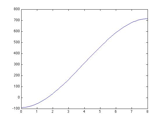
This function will return 0 when the value of h is such that the volume is 30. The function is a polynomial, so we can use either fzero() or roots(). To use fzero(), we need an initial guess. Graphing the function with fplot(), we see that there is a root in the vicinity of 2:

So we use 2 as the initial guess, and get an answer:

>> fzero(@spherevol,2,1e-6)
ans =
    1.6649
>>

Plugging this value back in, we get:

>> spherevol(ans)
ans =
  -1.4211e-14
>>

Which is quite close to zero. If we want to use roots(), we just need to create a vector of the coefficients of the 3rd-degree polynomial, and pass it to roots():

>> a = [-pi 3*pi*4 0  -3*30];
>> roots(a)
ans =
   11.7940
    1.6649
   -1.4590
>>

Note that the first adn last roots are not feasible, and the other is the same as we got with fzero().

(b) Fixpoint method. To use the fixpoint method, we have to define a new function, ff(h), such that whenever ff(h) = h, spherevol(h) = 0. This is easily done by simply adding h to the formula used in spherevol:

function y = ff(h)
    V=30;
    R=4;
    y = 3*pi*R*h^2 - pi*h^3 - 3*V + h;
end

Unfortunately, when we pass ff() to the fixpoint() function, we see that it diverges, for any guess close to the root:

>> fixpointwprint(@ff,2,1e-5,1)
Iter        x           g(x)           ea.         diff      slope
----   ------------  ------------   ---------      ----      -----
   0    2.00000000   37.66370614           Inf   35.663706   0.00
   1   37.66370614  -114423.18715802    0.94689848  114460.850864 3209.45
   2  -114423.18715802  4706927813334944.00000000    1.00032916  4706927813449367.000000 41122600242.03
   3  4706927813334944.00000000  -327614025741625546385314685577114629276111470592.00000000    1.00000000  327614025741625546385314685577114629276111470592.000000 69602517549879510446670593654784.00
ans =
   NaN
>>

This is because the magnitude of the derivative of the function in the vicinity of the fixpoint is much greater than one (we can either take the derivative and calculate its value at h=2, or we can plot the function and look at where it crosses the x=y line). We know that the fixpoint method will diverge under those conditions. So we need not try other guesses.

(c) Excel using "Goal Seek". It is straightforward to solve the problem using Excel. We don't have to rewrite the equation as f(x) = 0; we simply set up cells to contain h and R and V (where V is given by the equation in the problem), then set R to 4. Then we use Goal Seek to drive the cell containing V to 30 by varying h. A spreadsheet that shows the solution (along with the solutions to the other problems here) is here. Note that the solution is the same as that obtained with MATLAB to at least four decimal places.

Sphere volume problem with R=3, V=20. The same methods apply. We simply need to change the values assigned to the named constants in our functions spherevol() and ff():

    function y = spherevol(h)
       V=20;
       R=3;
       y = 3*pi*R*h^2 - pi*h^3 - 3*V;
    end

Using fzero(), with an initial guess of 1, we get 1.6073, which is the same answer we get with roots().

>> fzero(@spherevol,1,1e-5)
ans =
    1.6073
>> a = [-pi 3*3*pi 0 -3*20];
>> roots(a)
ans =
    8.7506
    1.6073
   -1.3579
>> spherevol(ans(1))
ans =
   1.3642e-12
>>

Before trying fixpoint(), we can plot the (modified) ff() function with the y=x line, to find the vicinity of the fixed point: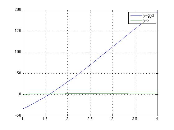

(The flatter line is y=x.) From this graph it is clear that the magnitude of the slope is too great to use the fixpoint method.

The Excel spreadsheet contains the solution for this equation also.

Amortization/Payment Problem.

Again we create a function from the equation, so that the function's value is 0 when its argument takes the value we want. From the given formula, we just want to move m over to the right-hand side, so:

     function y = amortf( n )
     P = 200000;  % principal
     r = 0.037;   % annual interest rate
     m = 1200;    % monthly payment
     y = P*r/(12*(1-1/(1+r/12)^n)) - m;
     end

This is not a polynomial in n, so roots() is not an option. With froot(), we see:

>> fzero(@amortf,240,1e-5)
ans =
  234.3015
>>

Using Excel, we get the same answer, i.e., 234.3 months. See the spreadsheet for the formulas.